Priya repairs laptops from a room above a shop in Thane. Customers send one-line complaints on WhatsApp, and by Friday the messages pile up faster than she can read them.
She keeps four of them in a text file to test a search box she is building.
my laptop battery drains in an hour.
laptop battery drains fast after the update and now the battery dies by noon.
the update killed my laptop speaker.
my laptop screen flickers when it is warm.
Then she types the three words she always types: laptop battery drains.
The first of those words cannot help her. Every message in the file is about a laptop. A word that appears in all four messages tells you nothing about which one to open.
That silence is the design.
A bag holds words, not sentences
Every search system, old or new, begins by turning text into numbers. The oldest way is to tip each message into a bag and count what falls out.
Word order goes first. In the bag, battery drains laptop and laptop battery drains hold the same three words. The bag cannot tell a question from an answer, or a complaint from its fix.
Grammar goes next. The bag does not know that drains is a verb in message one and a noun in a plumbing manual.
What is left is a small table. One row per message, one column per word that appears anywhere in the file, a number in each cell. Most cells hold zero.
That table alone ranks badly, because a long message beats a short one just by having more cells filled. Two corrections fix it, and the second is where the famous weight comes from.
What a word is worth
Start by asking how rare each word is. Count the messages that contain it. That count is the document frequency, and the first correction is to divide the number of messages by it, then take a logarithm.
weight = ln(messages in the file / messages containing the word)
With four messages the arithmetic comes out like this.
| Word | Messages containing it | Weight |
|---|---|---|
| laptop | 4 of 4 | 0 |
| my | 3 of 4 | 0.288 |
| battery, drains, update, the | 2 of 4 | 0.693 |
| fast, speaker, screen, hour | 1 of 4 | 1.386 |
Read the bottom row, then the top. A word in one message weighs 1.386. A word in half the messages weighs 0.693, exactly half. A word in three of four weighs 0.288. The word in all four weighs nothing, because the logarithm of one is zero.
Every time a word’s reach doubles, its weight halves, and a word that appears in every message is worth exactly nothing.
Nobody wrote a stopword list for that to happen. Nothing punished “laptop” for being boring. What punished it was sheer reach, and reach is a number you can count.
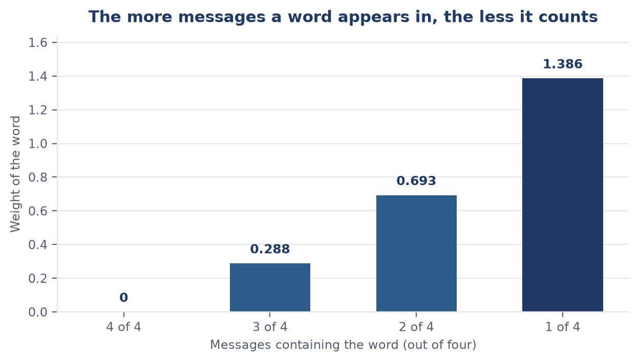
Each doubling of a word’s reach costs it half its weight. The rule needs no dictionary of English, only a message count.
Real collections look like this at scale. A small number of words sit in almost every document, and a long tail sits in one.
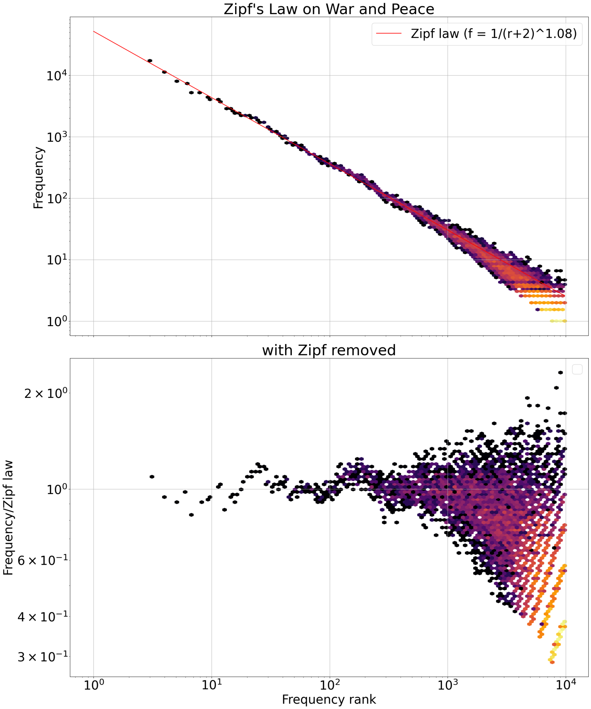
Every word in War and Peace, ranked by how often it appears. The fitted line is Zipf’s law, and the lower panel is what that line leaves unexplained. Image: Cosmia Nebula, CC BY-SA 4.0, via Wikimedia Commons.
Why take a logarithm
The first reason is the ladder. Reach doubles, weight halves, and the steps stay gentle enough to compare words whose reach differs by a thousandfold.
The second is arithmetic housekeeping. If you assume words appear independently, the chance of seeing two of them together is a product. Take logs and products become sums, so a document score can be the sum of one weight per word. Every ranking system after this one kept that shape. The base of the logarithm never matters, only the ratio inside it.
There is a popular story that this weight measures the information a word carries, in Shannon’s sense. Stephen Robertson went through those arguments in 2004 and found them wanting. His better answer: the weight is what a naive Bayes model hands you when you know nothing about which documents are relevant. It predicts relevance without ever being told what relevance is.
Four messages, scored
Score a message by adding the weights of the query words it contains.
Message one contains laptop, battery and drains. That is 0 plus 0.693 plus 0.693, so 1.386.
Message two contains the same three words, so 1.386 as well.
Messages three and four contain only laptop. Both score zero, correctly. One is about a speaker, the other about a screen, and Priya did not ask about either.
So the arithmetic returns a tie, and it shouldn’t. Message two is the one that says the battery dies by noon. It is also the only message that names the battery twice.
Count mentions as well as presence and the tie breaks. Inside message two, battery contributes 0.693 twice, so the message scores 2.079 against 1.386.
Message two wins, which is right. It wins by 50 percent, which is too much. It earned that lead by repeating a word, and it is twice as long as message one, fourteen words against seven. Two sloppy reasons to be confident.
The experiment that failed
In 1972 a researcher at Cambridge named Karen Spärck Jones published a short paper in the Journal of Documentation. She was trying to explain a failure of her own.
She had been grouping terms into clusters to help a search find more of what it should. The clusters kept getting taken over by terms that appear in many documents, and anything that made those terms match more documents pulled in noise with it.
The obvious fix was to delete them, and she tested that. On the Cranfield collection one term appears in 144 of 200 documents. Cutting frequent terms from INSPEC meant deleting 73 words of 1,341, and it lowered the ceiling on recall by at least 30 percent. On the Keen collection, recall fell from 75 percent to 25 percent.
People write requests in common words. In the Cranfield collection the average vocabulary term pointed at nine documents, while the average term used in a request pointed at 31.6.
So delete nothing, and pay the frequent words less. Her own version was cruder than the formula above: a whole number built by rounding to powers of two, with logarithms to base 2. On Cranfield’s 200 documents a term in 90 of them scored 2, and a term in 3 scored 7. She credits the smooth version we use today to Roger Needham, a Cambridge colleague.
She also notes how long it took to matter: AltaVista used this weighting from the start, about twenty-five years after the paper.
The paper justified its weights with a nod to Zipf’s law, and Robertson’s later analysis finds that argument weak. The measure outlived every explanation offered for it, including the one printed with it.
Where the other half of the name came from
The 1972 paper has no term frequency in it. That half came from Gerard Salton’s group at Cornell, who worked with abstracts and short texts, where how often a word appears inside one document carried signal. Salton and Yang published the combination experiments in 1973.
Two researchers, two kinds of data. Spärck Jones read presence and absence in word lists, so the number of documents was her variable. Salton read prose, so the number of mentions was his.
Multiply the two and you get tf-idf, though the multiplication was never derived from anything. It was assembled and then tested.
The ceiling
The last correction made this family of scores survive contact with real search engines. It is called BM25, published in 1994, and it adds one thing to tf-idf: a curve.
Counting mentions pays a flat rate forever. Six mentions are worth six times one. BM25 pays a lot for the first mention, less for the second, and approaches a ceiling it can never cross.
credit = (k1 + 1) × count / (k1 + count)
With k1 at 1.2, the value Lucene uses by default, one mention is worth 1.0, two mentions are worth 1.375, and ten are worth 1.964. The ceiling is 2.2 no matter how many times the word appears.
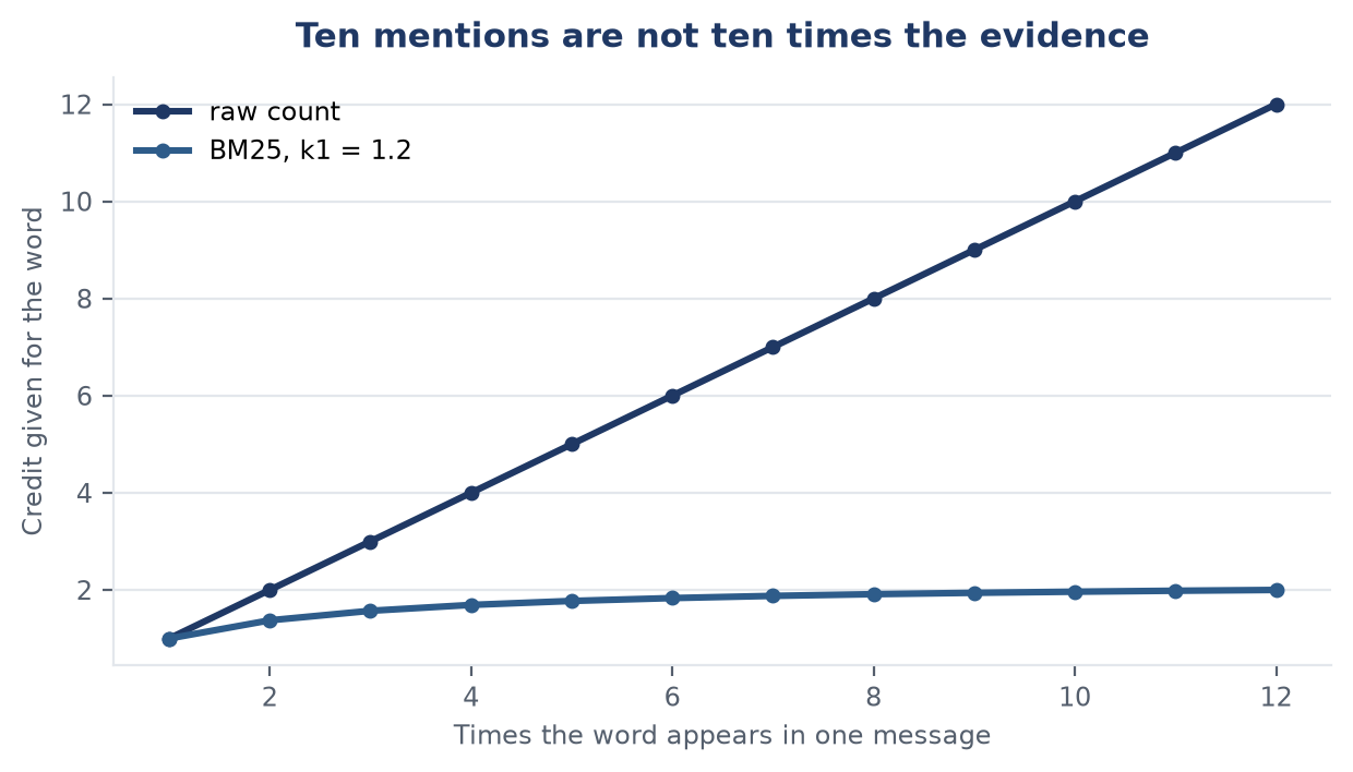
Raw counting never stops paying. BM25 gives the first mention most of the credit and then creeps towards a ceiling of 2.2.
Run Priya’s message two through that curve. Its doubled battery drops from 1.386 to 0.953, the message total falls from 2.079 to 1.646, and its lead over message one shrinks from 50 percent to 19 percent. The ranking does not change. The confidence behind the ranking does, and that is the honest thing to adjust.
There is a second dial for length, b = 0.75 by default, which discounts the length of a message against the average length of the collection. Message two is twice as long as message one, and that extra length earns it almost nothing.
Both dials were tuned by experiment. Robertson describes them as global parameters that are generally unknown and may be fitted to evaluation data, which is a polite way of saying the field guessed, measured, and kept what worked.
Still the baseline to beat
In 2021 five researchers at Darmstadt published BEIR, a benchmark of 18 retrieval datasets across nine tasks, and ran ten systems on them with no in-domain training. The average change in ranking quality against plain BM25:
| System | Average change vs BM25 |
|---|---|
| BM25 plus a cross-encoder re-ranker | +11.0% |
| ColBERT | +2.5% |
| docT5query | +1.6% |
| TAS-B | −2.8% |
| GenQ | −3.6% |
| ANCE | −7.4% |
| SPARTA | −20.3% |
| DeepCT | −27.9% |
| DPR | −47.7% |
Read the bottom row twice. DPR, a BERT-based dense retriever, averaged 47.7 percent below a formula with no neural network in it at all.
The cost is worse for the newcomers. BM25 answers a query over a million documents in 20 milliseconds on a CPU, with a 0.4 GB index. The winning combination needs 450 milliseconds on a GPU, or 6.1 seconds on CPU. On the 15-million-document BioASQ collection, ColBERT’s index runs to about 900 GB against BM25’s 18 GB.
The benchmark also flatters the old method. On the TREC-COVID dataset, 6.4 percent of BM25’s top ten had never been judged relevant or not, against 31.8 percent of TAS-B’s. When the researchers annotated 980 of those missing pairs by hand, ANCE climbed from 0.654 to 0.735, which put it 6.7 points above BM25 on the same data.
Both things hold at once. A formula from 1994, sitting on top of one from 1972, is a serious baseline, and the test sets that make it look unbeatable were built with formula-shaped tools.
What the bag cannot see
- Order.
battery drainsanddrains batteryare one bag. Addingnoto a complaint raises its score, becausenois another word in the bag. - Synonyms. A customer who writes
powerinstead ofbatterymatches nothing. Zero overlap, zero score. This gap is the entire reason dense retrieval exists. - Word relationships. Every word is scored on its own, so nothing in the model knows that
screenandflickersbelong to the same fault.
The library you will probably use gives numbers that do not match mine, and not because I made a mistake.
scikit-learn adds one to the top and bottom of the fraction before taking the log, as if it had seen an extra message containing every word. Its documentation says the effect is that words occurring in all documents “will not be entirely ignored”. So laptop comes out at 1.0 instead of zero, my at 1.223, a word in half the messages at 1.511, and a word in one at 1.916. The ladder survives. Only the zero disappears.
Robertson also notes that the older formulas, which keep the collection size on top, give a word in more than half the documents a negative weight, meaning its presence counts against you.
Try it on your own messages
Export a hundred of your own messages and count how many contain each word. Sort the list and look at the top twenty. You will find the words that describe your situation in general and none of your actual problem.
Then put two search words in reverse order and watch what your own search tool does with them.
Back to Priya
Her search box has never read a sentence of English. It has no idea what a laptop is, or that a battery dies by noon. It knows which words sit in which messages, and that in this particular file, this particular week, battery is worth paying for and laptop is worth nothing.
She types the three words she always types. Message two comes back first, and it should.
Relevance turns out to be mostly a question of what is rare in the room you are searching.