You have played this game. Somebody thinks of a person, a place or an object, and you get twenty questions to find it. Every question has to be answerable with a yes or a no.
Watch someone who is good at it. They do not guess. Their first question splits the world roughly in half, is it alive, and their second halves whatever is left. Someone who is bad at it asks whether the thing is smaller than a bus, rules out almost nothing, and has spent a question for free.
That instinct, the one you already have, is the whole algorithm behind a decision tree.
The only move it knows
A decision tree predicts by walking you down a chain of questions. Each one compares a single column of your table against a number: is the distance above twenty kilometres, is the hours-studied figure above four. You answer, you go left or right, you answer the next one, and wherever the chain runs out, the prediction is waiting.
A column here means one fact recorded for every row. Hours studied is a column. Whether a student turned up to lectures is another. The tree can ask about hours, and it can ask about lectures. It cannot ask whether the cost is more than twice the distance, because that question mixes two columns at once.
That restriction sounds like a weakness. In practice it is where most of the tree’s strengths come from, and most of its limits too.
Ten students walk into an exam
Ten students sat a mock exam. We know how many hours each of them studied, whether they attended lectures, and whether they passed.
| Hours studied | Went to lectures | Result |
|---|---|---|
| 1 | no | fail |
| 2 | no | fail |
| 3 | yes | fail |
| 4 | no | fail |
| 5 | yes | pass |
| 6 | yes | pass |
| 7 | no | fail |
| 8 | yes | pass |
| 9 | yes | pass |
| 10 | yes | pass |
Five passed and five failed. Student seven is the awkward one: seven hours of study, no lectures, and a fail anyway. Tables are full of rows like that, and the whole lesson of this article lives in what a tree does with them.
How mixed is this pile?
The tree builds itself by asking a question of its own at every step: which cut leaves the two new piles less mixed than the pile I started with?
So it needs a number for mixed. The usual one is the Gini impurity. Before any symbols, here it is in a sentence. If you picked two students out of a pile at random, how likely is it that one passed and the other failed?
Our ten students are five and five. Pick two at random and they disagree about half the time, so the pile scores 0.5. A pile of four students who all failed can never disagree with itself, so it scores 0. Everything else lands somewhere in between.
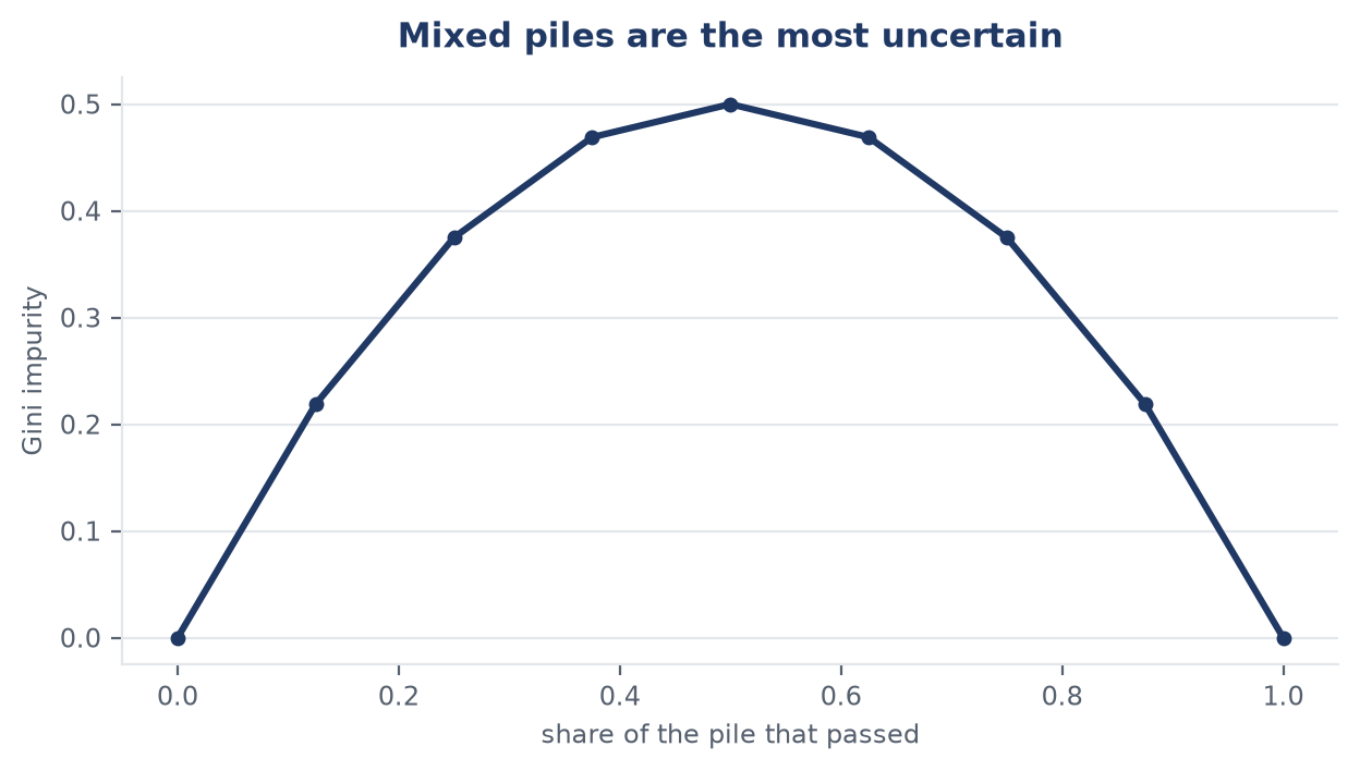
A pile where everyone passed is perfectly clean, scoring 0. A fifty-fifty pile is as mixed as it gets, scoring 0.5. Every cut is an attempt to move left along this curve.
The formula is Gini = 1 - (p1² + p2²), where p1 and p2 are the shares of each class in the pile. Take the share of passes, square it, take the share of fails, square it, add the two together, and subtract the total from one. Half and half gives 1 minus 0.5, which is 0.5. A single class gives 1 minus 1, which is 0.
The squaring is the useful part. It punishes small shares, so a lopsided pile scores low and a balanced one scores high.
The first cut
Now the tree tries every column at every threshold, and keeps whichever cut lowers that number the most.
Cut on hours, at four. The left pile is students one to four, all four of whom failed, so it scores 0. The right pile has one fail among five passes, which scores about 0.278. Combining them means weighting by size, four students left and six right, so 0.4 × 0 + 0.6 × 0.278 = 0.167.
The pile began at 0.5 and is now 0.167. That is a drop of 0.333.
Cut on lectures instead. The students who attended split into one fail and five passes, scoring 0.278. Those who skipped split into three fails and one pass, scoring 0.375. Weighted: 0.6 × 0.278 + 0.4 × 0.375 = 0.317. A drop of 0.183.
Hours wins, 0.333 against 0.183, so hours becomes the first question. Neither cut is clean, and that is fine. The tree only ever needs the cut that is best available.
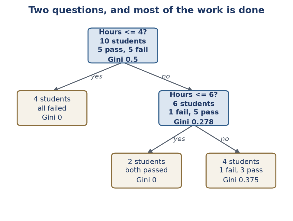
The first question does most of the work. The second buys a little more, and the box on the right is still mixed. One failed student is hiding in there.
The rule that exists to be wrong about one person
The leftover box holds four students, three passes and one fail. It is student seven again.
The tree can fix this. Ask one more question, hours at seven, and student seven drops into a leaf of his own: perfectly pure, impurity zero. The score improves. The model gets worse.
This is overfitting, and that single-row leaf is the disease in miniature. A rule whose only job is to be wrong about one student fewer on an exam you have already marked teaches you nothing about the next exam. Leave a tree to grow without limits and it will keep splitting until every leaf is pure, which on real data means roughly one rule per training row.
Every library gives you the same three brakes, and the defaults are loose enough that you get the overfitted tree unless you intervene. Cap the depth. Demand a minimum number of rows in each leaf. Or prune afterwards, charging the tree a fee for every leaf it keeps. If your leaves hold one or two rows, you did not fit a model. You indexed a spreadsheet.
What the tree is really doing to your data
Step back from the students and look at the shape of the thing.
Plot two columns as a flat sheet of paper. A question about hours is a vertical line. A question about lectures is a horizontal line. Every cut is a wall parallel to one axis or the other, and the leaves are the rectangular rooms those walls enclose.
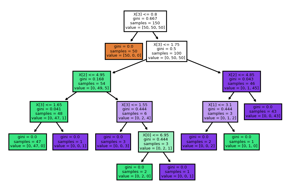
A real tree, trained on the iris dataset: 150 flowers, four measurements, three species. Do not bother reading every number. Look at the shape. A handful of yes-or-no questions is enough to separate three species almost perfectly. Image: Dvd8719, CC BY-SA 4.0, via Wikimedia Commons.
That picture explains what a tree cannot do. Suppose the rule is “pass if the hours and the attendance agree, fail if they disagree”, which gives you two diagonal stripes. No vertical or horizontal wall separates diagonal stripes, so the tree has to cut again and again, building a staircase to imitate a diagonal.
scikit-learn’s own documentation says so plainly: the algorithm is greedy, it makes the best-looking choice at each node, it cannot promise the best possible tree, and it struggles with concepts like XOR and parity. Greed is what keeps a tree fast and readable.
Why it still beats neural networks on spreadsheets
In 2022, three researchers assembled 45 datasets shaped like spreadsheets and tuned every model properly, neural networks included. Tree-based models still came out on top on medium-sized tables of around ten thousand rows, before anyone counted how much faster they run.
The explanation comes down to three things, and all three follow from the staircase.
Neural networks expect smoothness: nearby inputs should give nearby outputs. That is a gift for images. Tables are not smooth. A credit score of 699 is fine and 700 is refused. Trees expect nothing smooth, because they are flat by construction.
Neural networks also suffer when a table carries useless columns, since they have to spend capacity learning that a column is noise. A tree never picks it, because a useless column produces no gain.
And tables are built by people, one column at a time, so the useful directions already line up with the axes. Trees cut along those axes. Neural networks mix the columns together first and lose that alignment.
Quinlan’s 1986 paper on the ID3 algorithm has been cited around fourteen thousand times, which tells you how long this idea has been earning its keep.
Three things it cannot do
- It cannot extrapolate. Every prediction is the average of the rows that landed in that leaf, so it never returns a value beyond the range it saw. Show it a house twice as large as anything in training and it hands back the most expensive box’s average.
- It is twitchy. Change a few rows and the top question can flip, reshuffling everything below it. Two trees fitted on different halves of the same data can look unrelated. Averaging many of them into a random forest is the standard fix.
- Its probabilities are coarse. A leaf with three passes and one fail reports 0.75, which is a frequency taken from four students. Treat it as a rough ranking rather than a risk score.
Where to go next
A few good places, roughly in the order I would take them.
- Watch it drawn by hand. StatQuest: Decision Trees walks through impurity and splitting on a whiteboard in about seventeen minutes. If the Gini paragraph above felt slippery, this fixes it.
- Play with a real tree. explained.ai’s tree visualiser lets you change a split and watch the predictions move. It is the fastest way to feel what a cut does.
- Take the free short course. Kaggle’s Intro to Machine Learning is about four hours and ends with you training your own tree in a browser.
- Run the iris example yourself. scikit-learn’s decision tree plot is the picture from this article, generated by a short script you can copy.
- Read a book, if you want the maths. An Introduction to Statistical Learning is free to download. Chapter 8 covers trees and forests properly, and it assumes less than the title suggests.
The last question
Every model in the family, the forest and the boosted ensemble that wins most Kaggle tables and the ones with names you have not met yet, is a variation on one move: where do I cut?
Learn the tree as a staircase and the rest of the family reads as refinements of the same question.
So the next time an insurance form asks you five yes or no questions and then quotes you a price, you will know what just happened. You walked down a decision tree, and somebody chose where the walls go.